Clustering Lighthouses in Wikidata
Physical type k-means, k=4
Signal family k-modes, k=7
This map is formed from plotting the geographic locations of 5,625 lighthouses that were identified in Wikidata and processed through both K-mean and K-modes clustering. The lighthouses flash in real-time according to the light characteristic that is present in Wikidata.
The K-means clustering was performed on the physical properties of the lighthouses, while the K-modes clustering was performed on the signal characteristics of the lighthouses. Buttons at the top can be utilized to filter the visible lighthouses by combinations of k-means and k-modes clusters. Click on a lighthouse to bring up detailed information about it including an explanation of its properties as reported by Wikidata and a visual of the flash pattern of the lighthouse's signal.
1. Research Questions
Research questions
The questions that I came up with based on the properties in WikiData are:
- K-means: How do types of lighthouses resemble each other in physical form?
- K-modes: Do lighthouse signal patterns form a language, and does that language vary geographically?
Short answers
K-means: Lighthouses in the dataset fall into a few broad types that that have a significant amount of overlap. The main factor that separates clusters is the height of the light above sea level, with towers built atop cliffs being a clearly distinct grouping. In the remaining lighthouses the main component that affects cluster membership seems to be the height of the height of the constructed tower itself. Taller, long-range towers separate from short, limited-range ones though a significant amount of overlap muddies these two groups. A final group emerged that appears more defined by age rather than physical form.
K-modes: Going into this project, I did not know that the International Association of Marine Aids to Navigation and Lighthouse Authorities (IALA) provides guidance on lighthouse signals based on navigational needs in the area. Signals are already a designed code, so the k-modes mostly recovered its most common "words" (steady lights, single, double and triple flashes, quick flicker) rather than any real hidden grammar. There are indications of geographically defined clusters where it seems that IALA guidance is ignored, but these signaling differences are mixed in with those associated with more unique navigational needs. In the end, I believe that though signal patters do constitute a language of sorts for lighthouses, there is enough variation and nuance provided by distinct navigational challenges that K-modes clustering is not the right tool for addressing this question.
What this produces
The final presentation of this project is index.html and the associated imagry. This artifact comprises the data collection, written reflection, and visualization of the research conducted in this exercise.
A deployed version of this project is available on my personal site
Included in this repo are the raw datasets obtained from Wikidata and all source code for the pipeline that ultimately produces the refined data as CSV files, the images for elbow plots, and ultimately index.html.
2. Wikidata Queries
Querying
Full notes and (almost) every query are in data/Dataset Ideas.md.
This section is semi-interactive, if you want to engage with it. Each query used in this project is documented below along with a summary and the ability to run the query live against Wikidata and see the results.
QID Q39715 is the primary class identifier for all lighthouses. Different types of lighthouses are recorded as subclasses of Q39715. This query returns a list of every subclass and the count of items which are instances of that subclass.
SPARQL
SELECT ?class ?classLabel (COUNT(?item) AS ?n) WHERE {
  ?class wdt:P279* wd:Q39715 .     # same family tree
  ?item  wdt:P31   ?class .        # items that are an instance of that class
  SERVICE wikibase:label { bd:serviceParam wikibase:language "en". }
}
GROUP BY ?class ?classLabel
ORDER BY DESC(?n)
Many subclasses were excluded from the project. For example, sector lights (Q787078) are excluded as they are a different type of navigation aid and will not have the properties needed for this analysis. This query asks Wikidata how many items are an instance of any subclass of Q39715 that are not members of unrelated or unusable classes.
SPARQL
SELECT (COUNT(DISTINCT ?item) AS ?n) WHERE {
  ?item wdt:P31/wdt:P279* wd:Q39715 .     # instance of lighthouse, or of any kind of lighthouse

  MINUS {                                  # remove anything that matches this block
    VALUES ?excluded {                     # your exclusion list
      wd:Q787078 wd:Q1930418 wd:Q108840273 wd:Q33129345
      wd:Q66350506 wd:Q33129347 wd:Q33185258 wd:Q25324528
    }
    ?item wdt:P31 ?excluded .              # ...if the item is filed under any excluded class
  }
}
This query asks which properties the usable lighthouses have, and how many lighthouses have each property. This query was primarily used for identifying what properties would be useful for the two types of analysis used.
This query can run long and get timed out by the Wikidata query endpoint. This page runs a smaller query to retrieve properties for only a few subclasses.
SPARQL: as run for this project
SELECT ?prop ?propLabel (COUNT(DISTINCT ?item) AS ?count) WHERE {
  ?item wdt:P31/wdt:P279* wd:Q39715 .
  MINUS {
    VALUES ?excluded {
      wd:Q787078 wd:Q1930418 wd:Q108840273 wd:Q33129345
      wd:Q66350506 wd:Q33129347 wd:Q33185258 wd:Q25324528
    }
    ?item wdt:P31 ?excluded .
  }
  ?item ?p ?value .                        # ANY statement: the verb itself is a blank
  ?prop wikibase:directClaim ?p .          # translate the verb back to its property page, to get a name
  SERVICE wikibase:label { bd:serviceParam wikibase:language "en". }
}
GROUP BY ?prop ?propLabel
ORDER BY DESC(?count)
SPARQL: smaller version the Test query button runs
# Smaller version for the live test: only three kinds of lighthouse (caisson, wooden and
# Integral, about 240 items) instead of all 8,603, so it finishes inside Wikidata's 60 s limit.
SELECT ?prop ?propLabel (COUNT(DISTINCT ?item) AS ?count) WHERE {
  VALUES ?class { wd:Q5017835 wd:Q66088335 wd:Q3278565 }   # caisson, wooden, Integral lighthouse
  ?item wdt:P31 ?class .
  MINUS {
    VALUES ?excluded {
      wd:Q787078 wd:Q1930418 wd:Q108840273 wd:Q33129345
      wd:Q66350506 wd:Q33129347 wd:Q33185258 wd:Q25324528
    }
    ?item wdt:P31 ?excluded .
  }
  ?item ?p ?value .                        # ANY statement: the verb itself is a blank
  ?prop wikibase:directClaim ?p .          # translate the verb back to its property page, to get a name
  SERVICE wikibase:label { bd:serviceParam wikibase:language "en". }
}
GROUP BY ?prop ?propLabel
ORDER BY DESC(?count)
The properties I chose for K-means clustering were focal height above sea level for the light, construction date (inception), visible range of the light, height of the tower. Geographic coordinates and name (itemLabel) were included for mapping.
This query was heavily optimized by both Claude and Gemini as it repeatedly timed out. I do not understand the optimizations, but the results are what I expected.
SPARQL
SELECT ?item ?itemLabel ?coords ?focalHeight ?inception ?range ?height
WHERE {
  {
    SELECT ?item
      (GROUP_CONCAT(DISTINCT STR(?coord); separator=" | ") AS ?coords)
      (GROUP_CONCAT(DISTINCT CONCAT(STR(?focalAmt), " ", STRAFTER(STR(?focalUnit), "entity/")); separator=" | ") AS ?focalHeight)
      (GROUP_CONCAT(DISTINCT STR(?inception); separator=" | ") AS ?inception)
      (GROUP_CONCAT(DISTINCT CONCAT(STR(?rangeAmt), " ", STRAFTER(STR(?rangeUnit), "entity/")); separator=" | ") AS ?range)
      (GROUP_CONCAT(DISTINCT CONCAT(STR(?heightAmt), " ", STRAFTER(STR(?heightUnit), "entity/")); separator=" | ") AS ?height)
    WHERE {
      # 1. Restrict the base set as quickly as possible
      ?item wdt:P31/wdt:P279* wd:Q39715 .
      ?item wdt:P625 ?coord . # Bind coordinates immediately to drop non-geographic items

      # 2. Exclude your explicit classes
      MINUS {
        VALUES ?excluded {
          wd:Q787078 wd:Q1930418 wd:Q108840273 wd:Q33129345
          wd:Q66350506 wd:Q33129347 wd:Q33185258 wd:Q25324528
        }
        ?item wdt:P31 ?excluded .
      }

      # 3. Pull optional properties for the matched subset
      OPTIONAL {
        ?item p:P2923/psv:P2923 ?f .
        ?f wikibase:quantityAmount ?focalAmt ; wikibase:quantityUnit ?focalUnit .
      }
      OPTIONAL { ?item wdt:P571 ?inception . }
      OPTIONAL {
        ?item p:P2929/psv:P2929 ?r .
        ?r wikibase:quantityAmount ?rangeAmt ; wikibase:quantityUnit ?rangeUnit .
      }
      OPTIONAL {
        ?item p:P2048/psv:P2048 ?h .
        ?h wikibase:quantityAmount ?heightAmt ; wikibase:quantityUnit ?heightUnit .
      }
    }
    GROUP BY ?item
  }

  # 4. Apply labels at the very end to the reduced dataset
  SERVICE wikibase:label { bd:serviceParam wikibase:language "en". }
}
The categorical properties for lighthouses are very sparsely populated, and I wound up discarding most of the properties queried. Please see the "What didn't" section below for details.
This query was also heavily optimized by both Claude and Gemini as it repeatedly timed out. I do not understand the optimizations, but the results are what I expected.
SPARQL
SELECT ?item ?itemLabel
  (GROUP_CONCAT(DISTINCT STRAFTER(STR(?her), "entity/"); separator=" | ") AS ?heritage)
  (GROUP_CONCAT(DISTINCT STRAFTER(STR(?nrg), "entity/"); separator=" | ") AS ?energy)
  (GROUP_CONCAT(DISTINCT STRAFTER(STR(?mat), "entity/"); separator=" | ") AS ?material)
  (GROUP_CONCAT(DISTINCT STRAFTER(STR(?col), "entity/"); separator=" | ") AS ?color)
  (GROUP_CONCAT(DISTINCT STRAFTER(STR(?use), "entity/"); separator=" | ") AS ?hasUse)
  (GROUP_CONCAT(DISTINCT STRAFTER(STR(?lens), "entity/"); separator=" | ") AS ?lensType)
WITH {
  SELECT DISTINCT ?item WHERE {
    ?item wdt:P31/wdt:P279* wd:Q39715 .
    ?item wdt:P625 [] .
    MINUS {
      VALUES ?excluded {
        wd:Q787078 wd:Q1930418 wd:Q108840273 wd:Q33129345
        wd:Q66350506 wd:Q33129347 wd:Q33185258 wd:Q25324528
      }
      ?item wdt:P31 ?excluded .
    }
  }
} AS %lighthouses
WHERE {
  INCLUDE %lighthouses
  OPTIONAL { ?item wdt:P1435 ?her . }
  OPTIONAL { ?item wdt:P618  ?nrg . }
  OPTIONAL { ?item wdt:P186  ?mat . }
  OPTIONAL { ?item wdt:P462  ?col . }
  OPTIONAL { ?item wdt:P366  ?use . }
  OPTIONAL { ?item wdt:P9597 ?lens . }
  SERVICE wikibase:label { bd:serviceParam wikibase:language "en". }
}
GROUP BY ?item ?itemLabel
Assessing Wikidata
What worked
Wikidata queries provide a robust tool to retrieve a set of properties for thousands of instances of Q39715 and its subclasses. Standardization of units was easy due to cross referncing QID's that defined which unit values were stored in.
What didn't
The clustering algorithms for K-means and K-modes require all included records to have valid values for all fields used to fit the models. No N/A, no null values. This proved a major challenge for the K-modes analysis that I originally intended. I had chosen cultural heritage status, energy source, construction material, and color properties for K-modes. Of 8000+ lighthouses, only 58 have values for every field.
I repeatedly ran into timeout issues with many of the queries, which ultimately was solved by AI tooling which optimized the queries. Without access to those tools, I would almost certainly have changed project ideas.
Content in Wikidata is largely community-entered and community-maintained, which opens the platform up to a lot of biases that are inherent in volunteer created and maintained content.
What data went into each analysis
- K-means: 2,424 lighthouses, those with all four numeric properties: focal height, visible range, tower height, and construction year. Units were normalized, and the rows that had multiple values for the same property were reduced to one value.
- K-modes: 5,625 lighthouses. Since the categorical properties didn't work out, I used the light
characteristic (P1030) instead. This is a nautical chart code like
Fl(2) W 10s, so one field holds several categories. Each code was split into four fields: type (fixed, flashing, quick, etc.), group (flashes per group), color, and period. The period was binned (4s or less, 4-6s, 6-10s, 10-15s, over 15s, or none for fixed and quick lights). Codes that don't follow the standard notation were dropped.
3. How to run the code
NOTE: venv +
pip install -r requirements.txt(repo root; Python 3.12 tested). The Wikidata extracts ARE in the repo, so no network access is needed.
One command will run the full pipeline: python lighthouses.py
The individual steps are documented below:
| step | script | output |
|---|---|---|
| 1 | scripts/prep_kmeans.py |
data/k-means-lighthouses.csv |
| 2 | scripts/kmeans_lighthouses.py |
images/kmeans_elbow.png, data/output/kmeans_clusters.csv |
| 3 | scripts/prep_kmodes.py |
data/k-modes-features.csv |
| 4 | scripts/kmodes_lighthouses.py |
images/kmodes_elbow.png, data/output/kmodes_clusters.csv |
| 5 | scripts/map_clusters.py |
4 maps in images/ (needs steps 2 and 4) |
| 6 | scripts/scatter_clusters.py |
2 scatters in images/ (needs steps 2 and 4) |
4. K-means: physical form/age
Choosing k
The k-means data was fit at a range of k values and an elbow plot was generated.
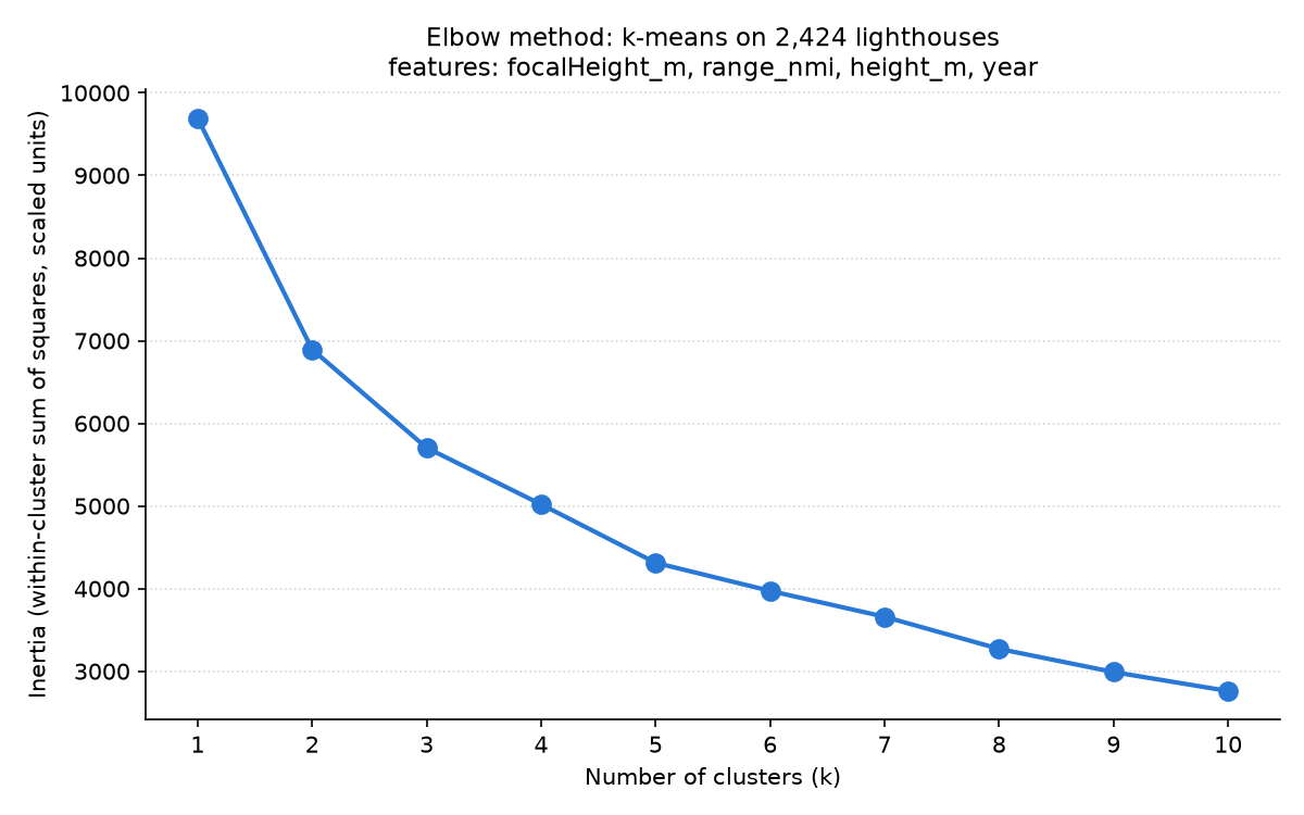
I struggled to find a compelling choice of k. Values 3, 4, and 5 were still quite steep with a long tail at higher k. I settled on k=4 for this analysis after inspecting the groupings at k=5. I felt like at k=4 the groupings were quite logical:
- A group for long-range lighthouses built atop cliffs
- A group for short towers with limited range
- A group for tall towers with long range
- A group dominated by older lighthouses
K=5 groups seemed to be less logical, and k=3 struggled to separate towers into useful clusters.
The four types
Values are the median for each cluster.
| Cluster | Lighthouses | Focal height | Range | Tower height | Year | Interpretation |
|---|---|---|---|---|---|---|
| 0 | 1,162 | 20 m | 11 nmi | 12 m | 1905 | small, short-range lights |
| 1 | 252 | 111 m | 21 nmi | 14 m | 1902 | short tower, very high lamp (likely cliffs) |
| 2 | 290 | 52 m | 23 nmi | 41 m | 1902 | tall towers close to water level |
| 3 | 720 | 37 m | 18 nmi | 20 m | 1866 | mid-size, older |
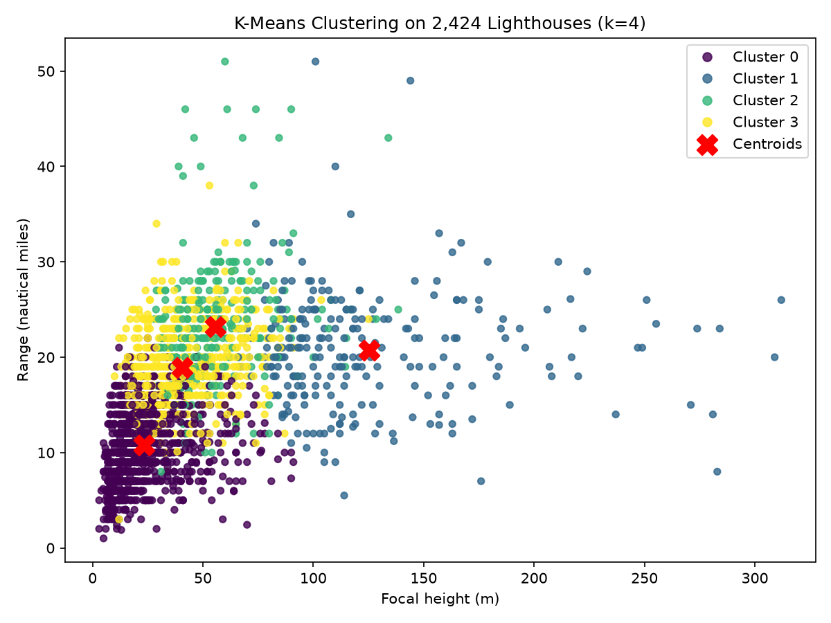
There is clear separation in this scatter plot between cluster 0 (small, short-range lighthouses) and cluster 1 (towers on cliffs), with very little overlap. This indicates that the fit model has good resolving power for which of these two groups a record belongs to.
In contrast, on the 2D scatter plot as generated, there appears to be a lot of overlap between cluster 2 (tall towers at water level) and cluster 3 (old towers of middle height). These records have similar heights and visible range of the light, but a significant 36 year difference in year of construction. If a 3D plot were made with the year as the additional axis, I suspect there would be obvious separation between the two clusters that is not visible with only two dimensions.
5. K-modes: light signals
Preparing the data
Claude was used to decode the maritime chart navigational light flash codes into the distinct data types used for analysis.
Some examples of light characteristic codes and how they ended up in the processed data:
| Code | What it means | type | group | color | period |
|---|---|---|---|---|---|
F R |
fixed (steady) red light | F | none | R | none |
Fl(2) W 10s |
white flashes in groups of 2, repeating every 10 seconds | Fl | 2 | W | 6-10s |
Iso WRG 4s |
equal on and off, white, red or green depending on direction, every 4 seconds | Iso | none | WRG | <=4s |
Fl(2+1) W 15s |
white group of 2 flashes then 1 flash, every 15 seconds | Fl | compound | W | 10-15s |
Choosing k
Like with k-means, an elbow plot was generated for a range of k values.
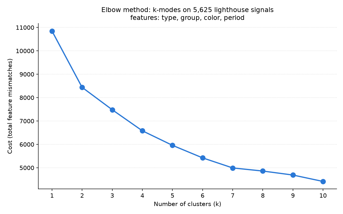
This chart has a more evident elbow at k=7.
Seven signal families
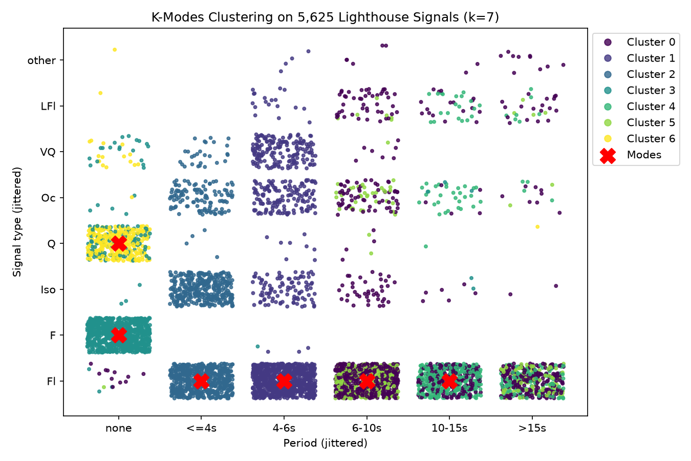
Each dot in this chart is a lighthouse, placed by its signal type and period and colored by which of the seven clusters k-modes put it in. Because these are categories, the dots are spread out randomly into blocks so you can see how many lighthouses share a signal, and the red X marks each family's most typical signal. At k=7 most blocks are a single color, so each family lines up with a recognizable signal.
In transparency, Claude suggested this chart. No example chart was included in the course demo, and I was struggling to tell if the groups made sense. This chart demonstrates that light signal patterns largely group together in k=7, with most of the overlap occurring in longer-duration flash cycles.
6. Bringing the two together
2,069 lighthouses made it into both analyses, so for those I can compare the physical type from k-means with the signal family from k-modes.
| Physical type | Lighthouses | Most common signal family | Fast flashes (4s or less) | White light |
|---|---|---|---|---|
| Small, short-range | 1,023 | medium single flashes (30%) | 23% | 62% |
| Cliffs | 186 | slow single flashes (46%) | 2% | 95% |
| Tall towers | 254 | slow single flashes (33%) | 6% | 90% |
| Mid-size, older | 606 | slow single flashes (37%) | 6% | 81% |
The two analyses line up more than I expected. The small, short-range lighthouses are where most of the variety is: they have almost all of the fast flashes (240 of 296), the steady lights and the quick flicker, and only 62% of them show a white light. The big lights are much more uniform. Lighthouses on cliffs are 95% white and almost half of them use a slow single flash, and the tall towers look similar. My guess is that this comes down to what each light is for: small lights mark harbors and channels where color and quick signals help, while the big lights need to be seen far out at sea.
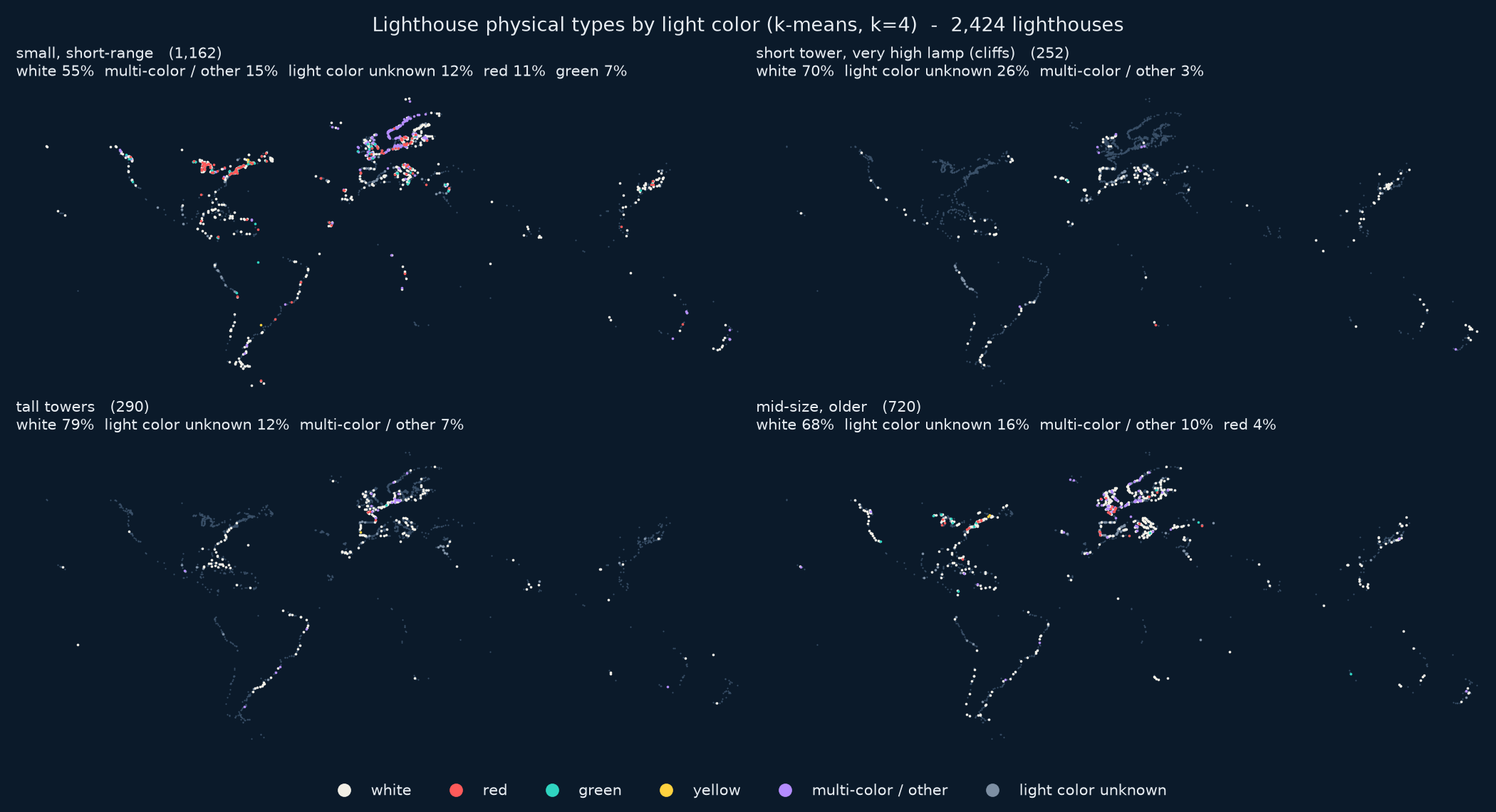
This map shows the light colors for each physical type. Its percentages are a bit different from the table because it also counts lighthouses that have no usable light characteristic.
7. Reflection
Decisions that shaped the results
A few choices I made along the way had a big effect on what came out:
- Binning the period. Splitting the flash period into bins is what created three of the seven k-modes families. Plain white single flashes ended up as three separate families (fast, medium and slow) only because of where I put the bin edges. Different bins would likely give different families.
- Normalizing the k-means features. Each feature was normalized, so all four k-means values count equally. This means a difference in construction year counts as much as a difference in focal height, which I think is part of why one cluster ended up being about age instead of physical form or location.
- Picking one value. About 1 in 6 of the k-means lighthouses had more than one value for some property, and I kept the largest range, the median height and the earliest year. Other rules could move some lighthouses into different clusters, but I do not think this affects a significant number of records.
- Picking one light code. 178 lighthouses have more than one light characteristic, and I used the first one that could be parsed. In practice this only changed the code for a few of them, so it barely mattered.
Limits of the tools
K-means is sensitive to extreme values. At k=5 it spends a whole cluster on just 15 very old lighthouses (median year 1543), which is part of why I didn't use k=5. The elbow plot also never had a sharp bend, so choosing the k value for the k-means analysis was a judgment call.
K-modes treats every mismatch the same. To the algorithm, a light that flashes every 5 seconds is just as "different" from one that flashes every 7 seconds as a flashing light is from a steady one. K-modes can also be thrown off by how the algorithm is initialized.
In this exercise I have learned that clustering is a powerful tool, but ultimately a very subjective one. Determining the "best" number of clusters to use for both analyses essentially boiled down to inspecting the values for each cluster and determining if the result felt good and seemed logical. What feels good and seems logical to me may be viewed very differently by another person.
Bias in the data
One look at the mapped locations of lighthouses in this dataset reveals several forms of bias that are built into the data itself. Extremely few inland lighthouses on rivers or lakes are present. I quite like the one Amazonian lighthouse in Brazil.
There is clearly a geographic bias present at the largest scale of this data. The global south is under-represented compared to the dominant European and North American data, despite the paths around southern Africa and South America being both heavily utilized and very dangerous.
I have no reason to suspect that there are genuinely fewer lighthouses in these areas. Instead, I suspect that Wikidata itself is biased toward the northern hemisphere and first-world countries.
Where the results are weak or ambiguous
- The k-means clusters 2D scatter plot shows a lot of overlap for two clusters. Tall towers and older towers look nearly the same on focal height and range, and the "older" cluster is defined more by age than by physical form.
- The k-modes families are loose. Only 25-53% of the lighthouses in each family exactly match its most typical signal, so most members only partly fit even if the groupings look good on the 2D chart.
- Lights with long cycles (over 15 seconds) don't have a family of their own and are split across three families.
- The elbow at k=7 isn't great. Though there is a diminished cost going from k=7 to k=8, the slope bends back down for k=9 to k=10. I did not explore the analysis in depth at a higher k.
- I only answered the geography part of my k-modes question by looking at the maps. I didn't test whether the regional differences are real or just reflect where Wikidata has more data.
8. AI disclosure
Claude and Gemini (via Google Search) were used in this project, particularly in the following areas:
- SPARQL query generation and optimization
- Javascript for charting the map at the top of the page
- CSS creation for styling
- Chart generation code for Matplotlib
- Live SPARQL queries in the HTML file
The bulk of the concept of this project along with the analysis, choice of k values, evaluation, and interpretation of the results are human-powered.